Just another bioinf blog
Blog by Michael Roach: @BeardyMcJohnFace@genomic.social
email: mroach@bioinf.cc
Circos part 2: Ribbons
08 Aug 2020
Following on from the previous post; in Circos part 2 I cover using ribbons to create a jupiter plot. In this example we make the plot from a nucmer alignment (part of the MUMmer package (https://github.com/mummer4/mummer)), using two different _Brettanomyces bruxellensis_ assemblies: AWRI2804 (https://www.ncbi.nlm.nih.gov/assembly/GCA_011074885.1) and CBS2499 (https://www.ncbi.nlm.nih.gov/assembly/GCA_000340765.1). The plots are great for visualising structural rearrangements and identifying potential misassemblies.Align the genomes
The first thing you’ll probably want to do is to rearrange your contigs for an optimal layout; I just used a script that I had on hand that wasn’t well suited to the task.
After arranging the contigs, we need to align the genomes, and it’s a good idea to also do a quick dotplot to see how things look. These alignments will be the ‘links’ that we plot in circos later.
# Do the alignment
nucmer -t 16 AWRI2804.oriented.fasta CBS2499.oriented.fasta

# Filter for 1-to-1 alignments
delta-filter -1 out.delta > out.1delta

# Make a dotplot
mummerplot --png --large out.1delta
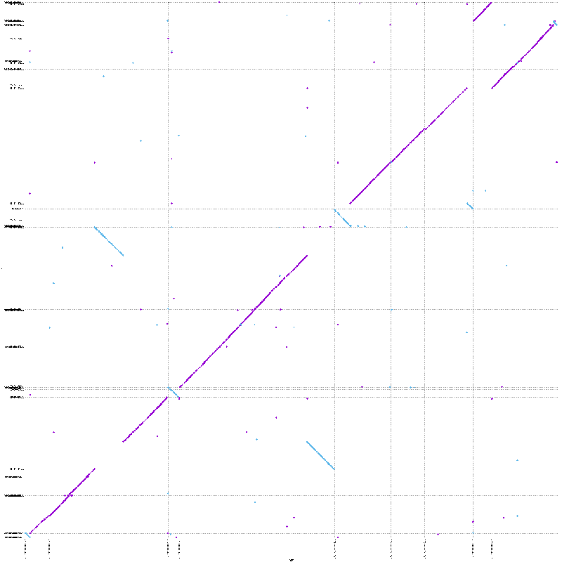
Quick fun-fact: you get a few files from mummerplot, but the fplot and rplot files are the forward and reverse alignments; you can plot these in R with some bash magic.
# bash terminal
# remove comment lines, add 'NA' breaks on blank lines
grep -v \# out.fplot | sed 's/^$/NA NA 0/' > ali.fplot
grep -v \# out.rplot | sed 's/^$/NA NA 0/' > ali.rplot
# R terminal
# read in the coords
fplt=read.table('ali.fplot')
rplt=read.table('ali.rplot')
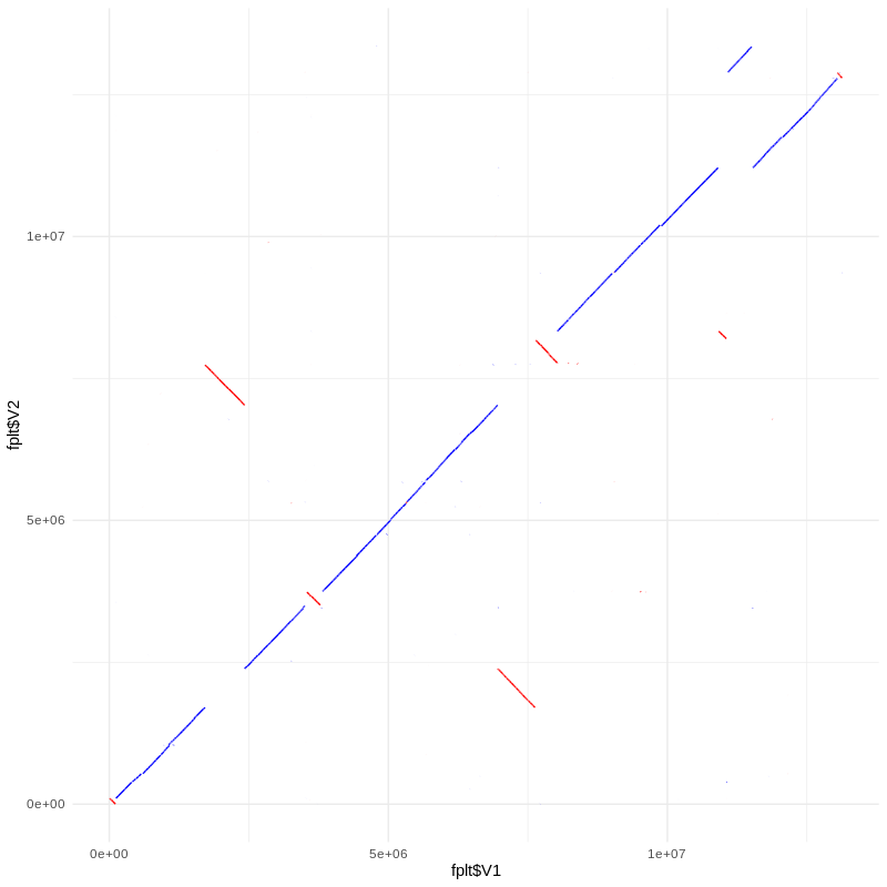
# plot with ggplot
library(ggplot2)
ggplot() +
geom_path(aes(x=fplt$V1,y=fplt$V2),color='blue') +
geom_path(aes(x=rplt$V1,y=rplt$V2),color='red') +
theme_minimal()
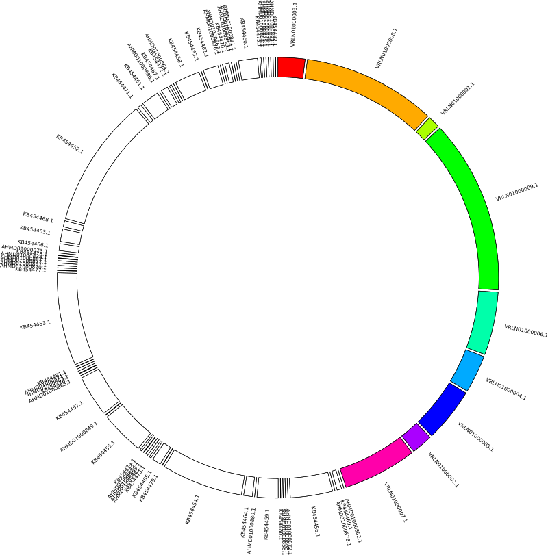
Karyogram
We make the karyogram the same way we did for part 1, only this time there are two assemblies which we’ll colour differently. You can specify colours as a hue, ranging from 0 to 360. Our reference (AWRI2804) has 9 contigs, so our hue ‘steps’ will be 360/9 = 40. The query (CBS2499) we’ll just colour white.
awk '{hue=sprintf("%03d", h); print "chr - "$1" "$1" 0 "$2" hue"hue; h+=40;}' AWRI2804.oriented.fasta.fai >  chr.kar
awk '{print "chr - "$1" "$1" 0 "$2" white"}' CBS2499.oriented.fasta.fai >> chr.kar
The circos configuration so far is essentially the same as for Part 1, but with some minor tweaks to get the contig names to fit better.
karyotype = chr.kar
chromosomes_units = 100000

<<include colors_fonts_patterns.conf>>
<<include housekeeping.conf>>

# IMAGE
<image>
<<include image.conf>>
</image>

# IDEOGRAM
<ideogram>
<spacing>
default = 0.5u
break = 1u
</spacing>
radius           = 0.75r
thickness        = 100p
fill             = yes
stroke_color     = black
stroke_thickness = 2p
show_label       = yes
label_radius     = 1.05r
label_size       = 30p
</ideogram>
And the ideogram should look like this:
Links/Ribbon
The links that circos plots will simply be the alignments that were generated by nucmer. You can view them with show-coords. We need to convert the format for circos so that the columns are:
refContig start stop queryContig start stop z-depth
We need to sort the alignments by alignment length so that we can apply a “z-depth”. Giving smaller alignments larger z-depths ensures that they are plotted on top of larger ones, which is better for overall clarity.
# bash terminal
show-coords -TH out.1delta | sort -k5,5nr | awk '{z+=1;print $8"\t"$1"\t"$2"\t"$9"\t"$3"\t"$4"\tz="z}' > links.tsv
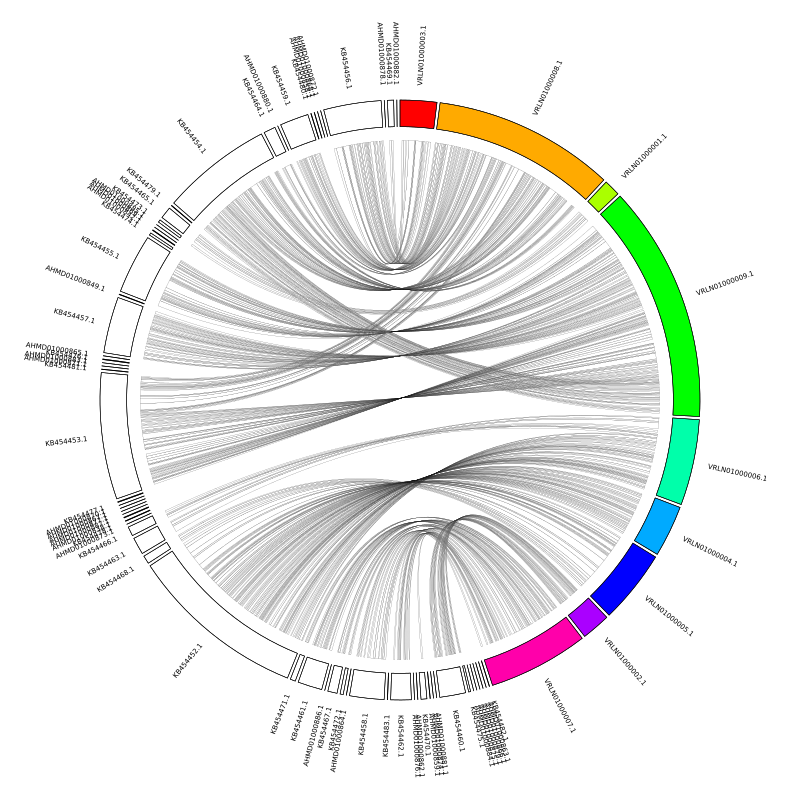
Add the config options for your links to your circos.conf file. There are two types of links that circos can make, we specify to use ‘ribbons’ with ribbon = yes. The default links are a set thickness and wont work that well for plotting alignments.
# LINKS
<links>
<link>
file                = links.tsv
radius              = 0.95r
ribbon              = yes
color               = white
stroke_color        = black
stroke_thickness    = 0.2p
</link>
</links>
Fixing the contig order
The first problem to address is that the alignments are all crossing over each other in the middle. What we want is for the query assembly to be mirrored against the reference. The contig order follows the order that we specify in the karyogram file, so we can simply remake this file with the query contigs listed in reverse order.
awk '{hue=sprintf("%03d", h); print "chr - "$1" "$1" 0 "$2" hue"hue; h+=40;}' AWRI2804.oriented.fasta.fai >  chr.kar
tac CBS2499.oriented.fasta.fai | awk '{print "chr - "$1" "$1" 0 "$2" white"}' >> chr.kar
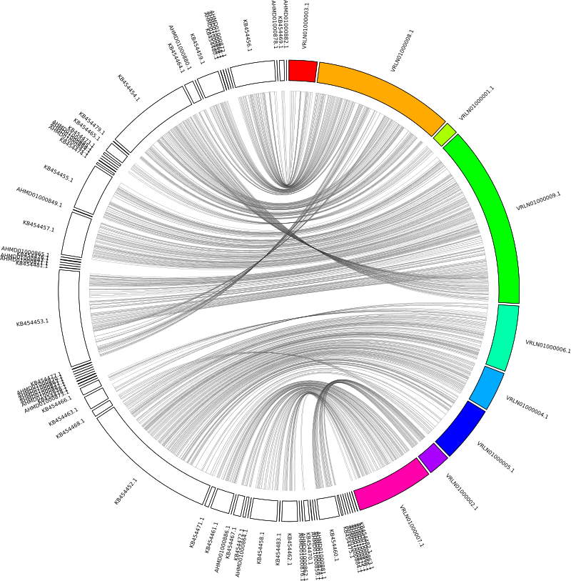
The next issue is that having reversed the contig order, all of our forward alignments now appear as reverse alignments. This is also easily fixed by telling circos to reverse the coordinates for the query contigs. We can specify individual contigs (e.g. chromosomes_reverse = contig1, contig2) or we can use regex. The query contigs have the prefixes ‘KB45’ and ‘AHMD’, so in the circos.conf we add:
chromosomes_reverse = /KB45/, /AHMD/
Add some colour
The last thing we need to do is colour the alignments according to the reference contig. It’s possible to specify the chromosome colours in the circos.conf file and map them with a rule, but it can be annoying if you have lots of contigs. You can specify the colour (as well as z-depth) in the links file. I find it just as easy to do this with a script that saves the chromosome colour mappings from the karyogram file to a dictionary, then parses the links file and appends the appropriate colour.
perl addCol.pl chr.kar links.tsv > newlinks.tsv
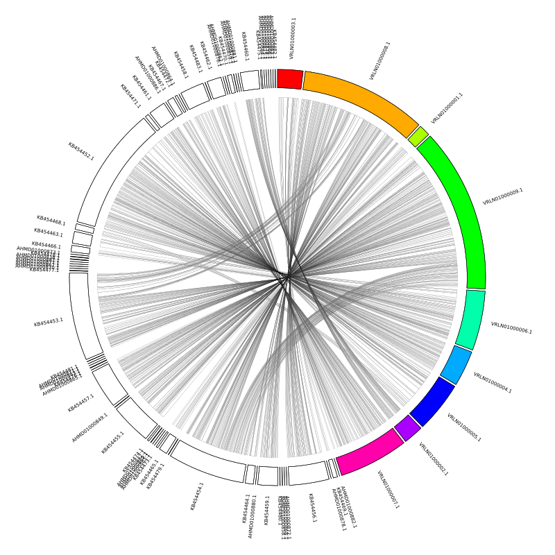
After updating the links file in circos.conf the plot should now look like this:
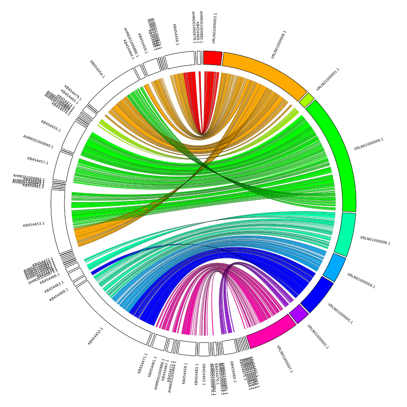
There are some interesting features and some contigs that a bit misplaced, and the Jupiter plot makes these very easy to spot.
Here are the final files used for the plot in case you wanted to try it out for yourself or use them as a reference: chr.kar; circos.conf; newlinks.tsv